Commissioning procedure for MCsquare
Contents
1. Overview
The Beam Data Library (BDL) is implemented in MCsquare as a look-up table containing parameters that characterize the beam for various energies. These parameters must be tuned to align the MCsquare simulation with experimental measurements. The commissioning procedure consists of several steps to be performed in a specific order:- Optimization of the BDL parameters
- Phase space:
Optical parameters such as the spot sizes and beam divergences need to be characterized at the nozzle exit. - Energy spectrum:
The spectrum is usually considered as Gaussian and is represented by a mean and standard deviation of the proton energy. - Absolute dose calibration:
The number of protons per MU is calibrated in order to compute absolute dose. - Validation of the generated beam model
2. BDL file format
The Beam Data Library (BDL) is a text file that describe the beam parameters. The first step of the commissioning process consists in generating a template of this BDL file, whose parameters will be adjusted during the optimization phases. Sample BDL files can be found in the BDL folder of MCsquare repository.The first line of the file “--UPenn beam model (double gaussian)--” indicates the format of the BDL to MCsquare. Therefore, it cannot be modified.
The next parameters provide the distance between the nozzle exit and the isocenter, then the distances between focal points (in x and y) and isocenter (SMX and SMY respectively), in millimeters units. Next, the number of energies to be commissioned must correspond to the number of rows in the following look-up table.
Finally, the look-up table provides all remaining parameters for each energy:
- NominalEnergy: the nominal energy (in MeV) as specified in the treatment plan.
- MeanEnergy: the actual mean energy (in MeV) that should be simulated to reproduce the proton range measured in water.
- EnergySpread: the standard deviation of the Gaussian distribution used to model the energy spectrum at the exit of the nozzle (in % of the nominal energy).
- ProtonsMU: the number of protons delivered per MU at this specific nominal energy.
- Weight1: the weight of the first Gaussian for the double Gaussian optical model. The sum of Weight1 and Weight2 should be 1.0.
- SpotSize1x: the in air spot size (in mm) along the x direction at the nozzle exit (for the first 2D Gaussian).
- Divergence1x: the spot divergence (in rad) along the x direction (for the first 2D Gaussian).
- Correlation1x: the correlation between the spot size and the divergence along the x direction (for the first 2D Gaussian). Its value must be between -0.99 and 0.99.
- SpotSize1y: the in air spot size (in mm) along the y direction at the nozzle exit (for the first 2D Gaussian).
- Divergence1y: the spot divergence (in rad) along the y direction (for the first 2D Gaussian).
- Correlation1y: the correlation between the spot size and the divergence along the y direction (for the first 2D Gaussian). Its value must be between -0.99 and 0.99.
- Weight2: the weight of the second Gaussian for the double Gaussian optical model. The sum of Weight1 and Weight2 should be 1.0.
- SpotSize2x: the in air spot size (in mm) along the x direction at the nozzle exit (for the second 2D Gaussian).
- Divergence2x: the spot divergence (in rad) along the x direction (for the second 2D Gaussian).
- Correlation2x: the correlation between the spot size and the divergence along the x direction (for the second 2D Gaussian). Its value must be between -0.99 and 0.99.
- SpotSize2y: the in air spot size (in mm) along the y direction at the nozzle exit (for the second 2D Gaussian).
- Divergence2y: the spot divergence (in rad) along the y direction (for the second 2D Gaussian).
- Correlation2y: the correlation between the spot size and the divergence along the x direction (for the second 2D Gaussian). Its value must be between -0.99 and 0.99.
3. Phase space
3.1 Measurements
The 2D fluence map of a single spot beam is measured in air for each commissioned energy. This measurement is repeated for N different distances from isocenter (at least N=3, including the isocenter itself, ahead of it and behind it). Examples of typical distances can be found in [1], [4].Fluorescent screen combined with a CCD-camera, such as the Lynx detector of IBA dosimetry, or flat panels are typically used for this measurement.
Note: It is recommended to verify the variation of the spot size at isocenter for different gantry angles. The full characterization of the beam shape is then generally performed at the gantry angle that provides an average spot size.
3.2 Post-processing method
The following procedure describes how to extract optical parameters (spot sizes, divergences, and correlations) at the nozzle exit from the measurement performed at the N different positions. The measured spot fluences can be modeled by single or double 2D Gaussian distributions. The procedure is explained for a single 2D Gaussian distribution, but it can easily be adapted for the double Gaussian case.- Perform a 2D Gaussian fit on the 2D fluence maps previously normalized to the volume under the surface.
- Extract the spot sizes σx(zi), σy(zi) (i.e. the standard deviations found at step 1) for i = 1, ..., N.
-
For each commissioned energy, perform two 1D fit of the Courant-Snyder formula using the spot sizes extracted at step 2:
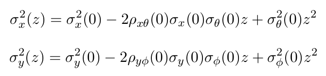
where z is the distance from isocenter, σθ the beam divergence in x direction, σφ the beam divergence in y direction, ρxθ the correlation coefficient in x direction and ρyφ the correlation coefficient in y direction.
These equations give the spot size at position z as a function of the spot size, divergence and correlation at isocenter (z=0). Since we measured spot sizes at N different positions, this can be used to retrieve the optical parameters at isocenter. The correlation coefficients must be constrained between -0.99 and 0.99. Note that the position z is supposed to be decreasing when moving away from the nozzle. For a divergent beam, divergence and correlation should be positive. For a convergent beam, it should be the opposite.
-
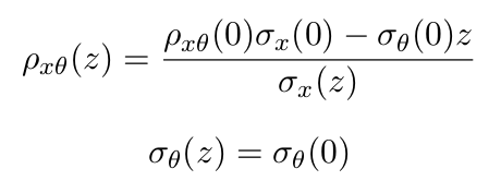
Once all parameters of Courant-Snyder equations are determined at the isocenter, the formula is used to extrapolate the optical parameters to the nozzle exit. Correlation and divergence can be found, for x, by using the following equations:
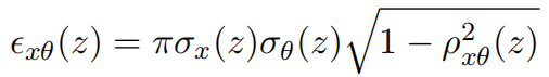
Note that the emittance, defined in Gate and MCsquare as the elliptic phase space area, can be obtained from the aforementioned optical parameters using the following formula (although different conventions on its definition exist elsewhere):
- Update the BDL file with the obtained values (6 per energy). The weight for the second Gaussian, in the BDL, is set to 0.0 for a single 2D Gaussian model.
4. Energy spectrum
4.1 Measurements
Energy spectrum parameters are extracted from integrated depth dose (IDD) profiles of single spot beams. These measurements are repeated for all commissioned energies. The acquisition is performed with large ionization chambers, such as the StingRay (IBA dosimetry) or the BraggPeak chamber (PTW), moving in depth inside a water phantom.4.2 Post-processing method
The proton energy spectrum is assumed to be a 1D Gaussian distribution. It is thus characterized in the BDL with 2 parameters (the mean and the standard deviation). These parameters must be tuned until the Monte Carlo simulation reproduces correctly the measured Bragg Peaks. This is repeated for each commissioned energy. The following procedure explain how to automatically optimize the energetic parameters.- Import the IDD measurements.
- Import a CT of water only (or any CT, choosing a HU calibration curve forcing water everywhere) and resample it to get a resolution of maximum 1 mm in depth (0.5 mm is preferred).
- Build a treatment plan in MCsquare format containing a single fraction, a single beam and a single spot (delivered at isocenter and with a weight of 1). The plan should reproduce exactly the measurement conditions
-
Use the following algorithm to optimize the mean energy and the standard deviation for each commissioned nominal energy:
- Adjust the energy in the plan with the current one.
- Normalize the measurements to the area of the Bragg peak curve.
-
Initialize the optimization with well chosen mean energy and standard deviation.
The easiest method consists in extracting the actual proton range r80, in cm, from the measured IDD curve and then to deduce the theoretical mean energy using the following formula fitted from the NIST/ICRU proton range database:
E0 = exp[3.464048 + 0.561372013 ln(r80) − 0.004900892 ln2(r80) + 0.001684756748 ln3(r80)].
In this case, the energy spread (standard deviation of the spectrum) can be initialized to 0.6.
Another method consists in performing a pre-optimization of the energy spectrum using a library of mono-energetic Bragg peaks pre-computed with MCsquare. A simple optimizer is used to find the best weight for each mono-energetic Bragg peak, so that the weighted sum reproduces the measured IDD curve. The weight distribution, hence describing the proton energy spectrum, is constrained to be Gaussian in order to extract the mean and standard deviation. This second method is slightly more complex to implement, but should be preferred as it provides a good initialization of both the mean energy and the energy spread.
-
Optimize the mean energy and the standard deviation of the proton energy spectrum by repeatedly running MCsquare simulations.
This step is time consuming because Monte Carlo simulations are performed at each iteration of the optimization. In order to limit the computation time, an efficient optimization algorithm and a good initialization of the parameters are required. The Nelder-Mead direct search algorithm is chosen for its efficiency. However, it does not always converge.
The optimizer is initialized with the mean energy and standard deviation obtained at the previous step. At each iteration, the objective function is evaluated as following:
- Update the BDL file with the current value of the optimized parameters.
- Run the MCsquare simulation with the plan created in step 3 and the updated BDL. In order to avoid any bias of the beam model caused by the noise inherent to Monte Carlo simulations, the statistical uncertainty on the results should be under 0.5%. Moreover, a special version of MCsquare, compiled with double precision calculation enabled, should be used.
- Integrate the resulting dose distribution over the detector area to obtain the IDD curve.
- Normalize the IDD curve to its area.
- Extract the metrics of interest from the normalized IDD. This can include the range 80, the FWHM, the dose-to-peak, ...
- Compute the error between the simulation and the measurement for each metric.
- Compute the objective function F defined as a weighted sum of these metrics. For instance:
F = 10 * error2range + (errordose-to-peak − errorFWHM)2
This is the function that is minimized by the optimizer in order to reproduce as good as possible the measurements with the MCsquare simulation.
If this optimization did not converge, a second optimization can be launched with an algorithm such as patternsearch. This last one is usually slower and less accurate than Nelder-Mead, but safer.
- Update the BDL file with the final solution.
- Adjust the energy in the plan with the current one.
5. Absolute dose calibration
5.1 Measurements
This step aims at measuring the absolute dose delivered per MU for each commissioned energy. These point measurements are performed in water, at a given depth in the middle of a uniform field (generally 10x10 cm2) using a small parallel plate ionization chamber, such as the PPC05.5.2 Post-processing method
In order to perform absolute dose calculation with the Monte Carlo simulation, the number of protons delivered per MU has to be determined. This value can be calculated for each proton energy by simulating the experiment described here-before and comparing the results with the absolute dose measurements. Here is the recommended procedure to extract the number of protons per MU:- Import the absolute dose measurements.
- Import a CT of water only (or any CT, choosing a HU calibration curve forcing water everywhere) and resample it to get a resolution of maximum 1 mm in (x, y). Set a depth resolution similar to the thickness of the active volume of your IC.
- Build a treatment plan in MCsquare format that reproduces exactly the measurement conditions (field size, number of spots, isocenter depth,...).
-
Use the following algorithm to compute the number of protons per MU for each commissioned nominal energy:
- Adjust the energy in the plan with the current one.
- Run the MCsquare simulation with the BDL obtained after the optimization of phase-space and energetic parameters. In order to avoid any bias of the beam model caused by the noise inherent to Monte Carlo simulations, the statistical uncertainty on the results should be under 0.5%. Moreover, a special version of MCsquare, compiled with double precision calculation enabled, should be used.
- Extract the mean dose over the detector area, at the measurement depth, from the simulated 3D dose map.
-
Calculate the protons per MU.
The measured dose per MU Dmeas normalized by the number of delivered protons Nprotons, meas should be the same as the simulated dose DMC normalized by the number of simulated protons Nprotons, MC :
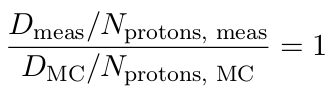
Therefore, the number of protons delivered per MU can be calculated with:
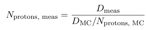
Note: The dose exported by MCsquare is provided in eV/g per proton. Unless you already use a post-processing method to convert the dose in Gy units, you will need to adapt the formula.
- Update the BDL file with the obtained protons per MU.
6. Range shifters
The definition of the range shifter can also be added in the BDL file, just before the number of energies and the look-up table. The definition of several parameters are required:
- Range Shifter parameters is a tag to notify the beginning of a new range shifter section.
- RS_ID is the name of the range shifter as identified in the dicom treatment plan.
- RS_type defines the type of range shifter (binary or analog). Note: only the binary mode is currently supported in MCsquare.
- RS_material defines the material composition for the range shifter. The parameter value is an unsigned integer representing the Material ID from the MCsquare material database (see Materials/list.dat). If your range shifter material composition does not exist yet, a new material will have to be generated in the database.
- RS_density defines the mass density of the range shifter (in g/cm3).
- RS_WET defines the Water equivalent thickness of the range shifter (in mm).
7. Validation
The validation can be performed in the same way as the validation of the TPS beam model. This should include at least the following checks:
- Relative dose verification of SOBP depth-dose profiles in water. This must be done for every commissioned energy, various field sizes, various range and modulation, various spot spacings, ... The range mainly but also the SOBP width need to be verified.
- Absolute dose verification in water. This must be done for every commissioned energy, various field sizes, various measurement depths, in the plateau and in the SOBP, various spot spacings, ...
8. References
[1] Fracchiolla F, Lorentini S, Widesott L, Schwarz M. Characterization and validation of a Monte Carlo code for independent dose calculation in proton therapy treatments with pencil beam scanning. Physics in medicine and biology. 2015;60(21):8601-8619.
[2] Goma C, Lorentini S, Meer D, Safai S. Proton beam monitor chamber calibration. Physics in medicine and biology. 2014;59(17):4961-4971.
[3] Grassberger C, Lomax A, Paganetti H. Characterizing a proton beam scanning system for Monte Carlo dose calculation in patients. Physics in medicine and biology. 2015;60(2):633-645.
[4] Grevillot L, Bertrand D, Dessy F, Freud N, Sarrut D. A Monte Carlo pencil beam scanning model for proton treatment plan simulation using GATE/GEANT4. Physics in medicine and biology. 2011;56(16):5203-5219.
[5] Huang S, Kang M, Souris K, Ainsley C, Solberg TD, McDonough JE, Simone CB II, Lin L. Validation and clinical implementation of an accurate Monte Carlo code for pencil beam scanning proton therapy. Journal of applied clinical medical physics. 2018;19(5):558-572.
[6] Kimstrand P, Traneus E, Ahnesjo A, Grusell E, Glimelius B, Tilly N. A beam source model for scanned proton beams. Physics in medicine and biology. 2007;52(11):3151-3168.
- Adjust the energy in the plan with the current one.